A cash forecast can look accurate at the terminal level and still produce an avoidable outage. The usual reason is denomination imbalance: the ATM has enough value on hand, but the cassette holding the notes customers request most often reaches its minimum before the next service visit. To configure ATM cassette forecasting effectively, operations teams need to forecast demand, physical capacity, service timing, and denomination mix together.

For a fleet manager, the objective is not simply to predict withdrawal volume. It is to keep each terminal serviceable through its planned visit window while limiting excess cash, emergency calls, and unnecessary route miles. The best configuration is therefore specific to the location, cassette layout, replenishment model, and the quality of available transaction data.

Start with the operating decision

Forecasting settings should reflect the decision the system is expected to support. A forecast used to flag same-day emergency replenishment needs different tolerances from one used to build a weekly cash route. Mixing those purposes often creates noisy alerts and encourages planners to distrust the model.

Define the forecast horizon first. For a daily serviced branch ATM, one to three days may be enough. A retail fleet with twice-weekly armored-car visits may require a five- to seven-day forecast, including a safety margin for missed service windows. The horizon must extend beyond the nominal schedule when route disruptions, holiday closures, or weather events are credible risks.

Then define the operational action tied to the forecast. A cassette projected to reach a minimum level should trigger a proposed replenishment, a route review, or an escalation only when there is time to act. Alerts that arrive after dispatch cutoffs may be technically correct but operationally irrelevant.

Configure ATM cassette forecasting by cassette, not value

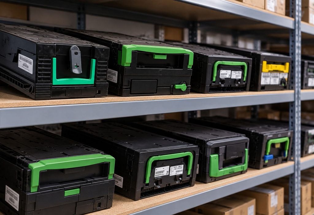
A terminal-level cash balance is a weak control measure. An ATM with $40,000 remaining may be unable to satisfy a common $100 withdrawal if its $20 cassette is depleted and only $50 notes remain. Configuration should therefore model each dispensing cassette as its own inventory position.

For each cassette, record the denomination, usable note capacity, initial load, reject and purge behavior, and any notes reserved for operational purposes. Usable capacity matters more than the manufacturer’s nominal cassette capacity. Note condition, cassette mechanics, local loading practices, and retained notes can reduce the number of notes that can be safely loaded or dispensed.

The model also needs to recognize the ATM’s dispense logic. Some terminals dispense a preferred mix, while others use rules designed to preserve a denomination, minimize note count, or meet customer-selected denominations. A change in dispense algorithm can materially alter cassette consumption even when total withdrawal dollars do not change.

This is particularly relevant as fleets introduce denomination choice or support mixed withdrawals across $10, $20, $50, and $100 notes. Historical cash demand remains useful, but only if it is recalculated after changes in customer options or dispense rules. Assuming that the old denomination pattern will hold can cause a new cassette mix to fail quickly.

Build the baseline from usable transaction history

The baseline forecast should use completed dispenses by denomination where that data is available. If the system records only transaction value, the forecast must infer note consumption from dispense logic, which is less precise and should carry a wider safety stock.

A practical starting period is 8 to 13 weeks of clean history. That range usually captures weekly patterns without giving too much influence to behavior that no longer reflects current traffic. However, a site with highly seasonal demand may need a longer reference period, with seasonal periods treated separately rather than averaged into ordinary weeks.

Clean the data before setting parameters. Exclude periods when the terminal was out of service, cash-out, communications-impaired, or operating with an unusual cassette configuration. A cash-out is not evidence of low demand. It is evidence that demand became unobservable after the relevant cassette emptied.

Likewise, distinguish true demand spikes from operational artifacts. A nearby branch closure, a payroll event, a festival, or a temporary fee change may justify an adjustment. A one-time loading error should not become part of the baseline.

Account for day-of-week and pay-cycle effects

Most ATM demand is not evenly distributed. Friday, weekend, month-end, and benefit-payment cycles can shape both transaction counts and denominations. A site near a stadium, transit center, military installation, or cash-intensive retail corridor may have a pattern that differs sharply from the surrounding fleet.

Forecasting configuration should use daily profiles where data supports them. At a minimum, assign separate expected consumption rates for business days, weekends, and known high-demand dates. Treating every day as average is one of the fastest ways to overfill slow locations and understock busy ones.

The model should also allow planners to enter justified event overrides. These should be time-bound and reviewed after the event. Permanent manual uplifts tend to accumulate, obscure model performance, and tie up working cash.

Set minimums around service risk, not arbitrary percentages

Many operations use a fixed cassette threshold, such as 20% remaining. That is easy to administer but rarely aligned with actual risk. A 20% threshold may be excessive for a low-volume branch terminal serviced daily and inadequate for a high-volume off-premise location before a holiday weekend.

A better minimum is based on expected consumption until the next realistic replenishment opportunity, plus a safety stock. The safety stock should reflect demand variability, forecast error, and service uncertainty. Sites with stable weekday behavior and reliable daily service can operate with smaller buffers. Sites with variable demand, long routes, or frequent service exceptions require more protection.

Consider the cutoff time as part of the calculation. If an armored-car route must be finalized at 2 p.m., a cassette forecast at 4 p.m. cannot prevent a next-day shortage unless an exception service option exists. The planning system should evaluate projected inventory at the point where a route decision must be made, not only at the scheduled arrival time.

Maximum settings deserve equal attention. Loading every cassette to capacity may reduce service frequency, but it increases idle cash, can distort route planning, and may exceed risk limits. The right target load is often the amount needed to cover the forecast horizon and buffer, rounded to practical strap quantities and within approved cash exposure limits.

Add real-world service constraints

Forecast quality is only half the problem. The configuration must incorporate the service model that turns forecasts into action. Record scheduled visit cadence, permissible visit days, route cutoffs, holiday restrictions, branch access hours, and the lead time for emergency service.

For managed fleets, route capacity can be a binding constraint. A forecast may recommend 40 stops on a day when the carrier can complete 30. In that case, prioritize locations by projected stock-out time, customer impact, alternate-channel availability, and the possibility of rebalancing denominations at nearby terminals. A forecasting engine that ignores route capacity can produce a technically sensible but unusable worklist.

Cassette swaps also affect the configuration. If field teams exchange sealed cassettes rather than count and replenish notes at the terminal, forecasting should use the inventory and availability of prepared cassettes. A predicted need is not actionable if the required denomination cassette has not been staged at the depot.

Test exceptions before relying on automation

Cash forecasting should not be treated as a set-and-forget rule. Configure exception handling for partial dispenses, cash-present events, reject spikes, cassette low states, note jams, and feed failures. These events can make the electronic cash position diverge from the physical position.

Reconciliation data is essential. Compare predicted cassette balances with verified balances at every service event, then measure error by terminal, denomination, day type, and forecast horizon. A fleet-wide average can hide a small group of consistently inaccurate sites that generate most emergency activity.

When error is persistent, investigate the cause before increasing safety stock. The issue may be a dispense-log mapping problem, an incorrect cassette capacity, a software configuration mismatch, or a location whose demand behavior has changed. More buffer can contain the symptom, but it increases cash exposure and may leave the underlying data problem untouched.

Roll out in controlled stages

A sensible rollout starts with a representative group of terminals: stable branch sites, variable retail locations, and several high-volume machines. Run the forecast alongside current planning for several service cycles. Compare projected and actual note consumption, proposed loads, stock-out risk, and route implications before allowing automatic recommendations to drive dispatch.

Parameter governance matters as the fleet grows. Limit who can change denomination mapping, thresholds, demand overrides, and service calendars. Every change should be traceable, especially when an adjustment affects cash exposure or explains a missed service target.

The strongest cassette forecasting programs remain operationally curious. A forecast should prompt a useful question at the right time: is demand changing, is the service cadence wrong, or is the cassette mix no longer appropriate for this location? That discipline turns cash forecasting from a reporting feature into a practical control for availability and cost.